Cornell Summer School Notes
1 Overview: Goals and Objectives
Many of you are creating languages for capturing networking concepts. Since you’re at this workshop, you might be interested in applying formal methods to your languages. Our session is designed to help you think about what good formal methods can do for network maintainers, how you can map a configuration language into formal methods, and issues to consider when designing a language for analyzability.
2 Margrave (40 minutes)
Our session has two high-level goals: we want to introduce to you our configuration analysis tool, called Margrave, and we want to help you start thinking about how formal methods tools can support configuration analysis.
2.1 Writing Configurations in Margrave
Let’s start with a simple example of a packet filter in a system with a server at IP address 10.1.20.20. Here is the behavior we want :
Packets to the server from the machine at IP address 10.1.1.2 should be denied
Packets from other machines to the server should be allowed
Packets to port 80 should be denied unless they are sent to the server
All denied packets should be logged
Margrave is designed for capturing configurations that are made up of rules. Each rule captures the decision that the rule renders and a set of conditions that can yield that decision. Start with our first requirement, that the filter should reject packets from 10.1.1.2 to the server. In Margrave, we would write this as
rule1(deny(sa, sp, da, dp) :- =(sa, $10.1.1.2), =(da, $10.1.20.20))
"rule1" names this rule (we’ll see why this is useful later). "deny" is the decision, which is based on the four inputs "sa", "sp", "da", and "dp" (for source address, source port, destination address and destination port, respectively). The :- separates the decision clause from the conditions for rendering the decision under this rule: in this case, the source address must be equal to 10.1.1.2 and the destination address must be equal to 10.1.20.20. The equality operator uses prefix notation. The IP addresses have $ in their names to denote that they are constants (rather than variables) in Margrave.
Now look at the second requirement, that packets from other machines should be allowed. The rule structure is the same, though the decision in this case is "permit", and the source address is not a specific address:
rule2(permit(sa, sp, da, dp) :- =(da, $10.1.20.20))
Before we capture the rest of the requirements, let’s understand how Margrave would interpret a configuration containing these two rules (in other words, what is the semantics of rules and configurations in Margrave). We’ll discuss this intuitively, showing you the formal syntax for making and querying configurations a bit later.
Imagine that someone asked whether a packet from 10.1.1.2 to the server at 10.1.20.20 is denied. Margrave checks each rule against the request to see if one produces a deny decision on that packet. Yes, the first rule does.
What if we asked whether a packet from 10.1.1.2 to 10.1.20.20 is permitted? Again, Margrave checks each rule against the request to see if one produces a permit decision on that packet. Yes, the second rule does. Nothing in the second rule says that the source address can’t be 10.1.1.2, so the rule applies.
Isn’t this a problem? It seems to suggest that Margrave allows configurations to return conflicting decisions. Real systems shouldn’t do that, right?
This question reflects an essential difference between analyzing and deploying configurations. Sometimes, people write configurations with conflicting rules, or missing cases, or with one rule unexpectedly shadowing another. Analysis helps you identify and correct those situations before you deploy the configuration. We want Margrave to observe conflicting decisions (if they exist) because that helps us get to a better configuration before deployment.
Okay, but having found the conflict, we would like to resolve it and have Margrave analyze the resolved configuration. Some configuration languages support priorities among decisions: if the individual rules would allow two decisions, the priorities determine which decision is actually rendered. Others base the decision on the order in which rules are listed in the configuration: the earliest applicable rule applies. Margrave supports both mechanisms. Packet filters typically follow the first applicable discipline. We will add the following statement indicating this to our configuration:
RComb(fa(permit, deny))
Here, "RComb" stands for "rule combinator". Read this line as "take the first applicable decision among permit and deny".
Now that you have a sense of how Margrave evaluates rules, let’s finish adding rules for the rest of our desired behavior.
Exercise: Write rules to capture the third and fourth requirements. Use the constant $port80 to refer to the web port.
Let’s start with the third requirement. Note that the requirement implicitly contains two rules, one to deny and one to permit. So we should capture this with a pair of rules:
rule3(deny(sa, sp, da, dp) :- =(dp, $port80)) |
|
rule4(permit(sa, sp, da, dp) :- =(dp, $port80), =(da, $10.1.20.20)) |
The rule to log denied packets requires that we introduce a new decision corresponding to logging. Intuitively, decisions capture any action that should get reported as output of the configuration. If we have a log decision, we could capture this requirement with the following rule:
rule5(log(sa, sp, da, dp) :- deny(sa, sp, da, dp))
Although "deny" is a decision, this rule uses it as a condition for the "log" decision. Margrave has some restrictions on how you use decisions as conditions in other decisions (for example, you can’t use deny to define deny).
Now that we are also using a log decision, let’s look at our rule combination statement again:
RComb(fa(permit, deny))
Note that it mentions only permit and deny, not log. Should we change it to reference log? No, because we want log to get reported along with deny (log and deny simultaneously is not a conflict among decisions, unlike permit and deny). Margrave lets rule combination omit decisions, precisely for situations like logging.
By now, you might be wondering how Margrave knows about the various terms that we’ve used in writing these rules. Our rules refer to decisions (permit, deny, log), IP addresses ($10.1.1.2), and ports ($port80), but we don’t seem to have defined these terms anywhere. In fact, every Margrave configuration comes in two parts: one part containing the rules and conflict resolution, and another that sets up the decisions and concepts that will appear in these rules. Each part lives in its own file, the rules in a .p file ("p" for "policy"), and the setup in a .v file ("v" for "vocabulary"). We won’t go into the structure of these files in detail here for sake of time, but we will look at some highlights [here are the files: filter.p | filter.v]:
The .v file states the type names for the spec (here, IPAddress and Port).
The .v file introduces constants for specific IPAddresses (e.g., $10.1.1.1(IPAddress)) and Ports (e.g., $port80(Port)). Margrave does not automatically understand IP addresses—
we manually introduce addresses we want to work with in the .v file. The Axioms section of the .v file states constraints or invariants on the vocabulary data. In this case, we say constants-neq-all(IPAddress) to capture that each IPAddress is unique (similarly for ports). By default, Margrave allows two constants to refer to the same object in a scenario: constants-neq-all tells Margrave to force each constant in the given type to refer to a distinct object.
The .p file indicates the vocabulary it needs in the uses clause at the top of the Policy declaration.
The Variables section of the Policy defines the inputs that make up a request to the rules in the configuration. Each variable has a name and a type.
Separating the .p and .v files allows the same vocabulary to be used for multiple configurations. We’ll see an example of how this is useful a bit later.
Time to summarize. At this point, you should understand:
Margrave supports configurations written in terms of rules
Multiple rules can apply to the same inputs. Rule combinators let you specify when and how to resolve multiple decisions into a single decision
Rules go into one file, written in terms of domain-specific concepts
Domain-specific concepts are defined in another file that can be reused across configurations
How does Margrave’s input language compare to Alloy, or a generic SAT solver? Margrave is tailored for constructs needed to write rule-based configurations. You certainly could write configurations against either Alloy or formulas (as needed for SAT solvers), but Margrave provides constructs geared towards that task.
Exercise: Take a stretch break
2.2 Analyzing configurations in Margrave
Now that we have our packet filter written in Margrave, let’s use Margrave to analyze it. We’ve already discussed one question one might want to ask about a configuration, namely "will the filter allow/reject a specific packet". Let’s brainstorm a bit: what questions might you want to check of a packet filter?
Exercise: Write down at least one other question you might want to ask about a packet filter
Here are some possible answers:
Will the filter allow a specific packet?
Are any source ports from which packets are always rejected?
What are all the ports from which a packet might be permitted?
Are there any redundant rules in the filter?
What rules could I add to allow packets from a particular set of machines to reach a server, but without changing the decisions of other packets?
The first three are questions about the observable behavior of the filter. The fourth is a question about the structure of the filter itself. The fith asks about how to edit the filter to achieve specific goals.
Whenever you set out to design formal analysis techniques for a particular setting, start by asking yourself which analysis questions you want to let someone ask. The set of questions helps determine which methods you can use, which data structures you need, etc.
Margrave handles the first four questions, but not the fifth. In this segment, we’ll show you how to do queries like the first four, and develop your intuition about why the fifth is harder.
Let’s start with a basic query: what WWW traffic does the filter allow? We can write the query as follows:
let q1[sa: IPAddress, da: IPAddress, sp: Port, dp: Port] be |
filter:permit(sa, sp, da, dp) and dp=$port80 |
Here, "q1" is the name of the query. After the name of the query, we list the parameters for the query (in square brackets). Each parameter has a name and a type, with the type coming from the vocabulary. After be, we write a boolean formula with the criteria for the query. In this case, we want a permit decision with the destination port being port80. Unlike the Margrave policy language, the query language does support infix for equality.
The let construct defines a query, but doesn’t run it. To run it, we use the show command:
show q1
This asks Margrave to produce scenarios that illustrate the query. Margrave produces one scenario at a time. We can see additional scenarios by repeating the command show q1. If you want to start the iteration afresh, use reset q1.
What does a scenario look like? Here’s one for q1:
--***-- SOLUTION FOUND at size = 7. --***-- |
da=$10.1.20.20: IPAddress |
dp=$port80: Port |
sa: IPAddress |
sp=$port25: Port |
IPAddress#1: IPAddress |
----------------------------------------------- |
The scenario involves several ports and IP addresses, some of which correspond to the variables in the query. This scenario has a packet to the server (the da=10.1.20.20: IPAddress line), coming from an arbitrary source address (the sa: IPAddress line (we know it is arbitrary because the scenario does not provide a specific value for sa). The scenario also included an arbitrary IP address IPAddress#1 that was not bound to any variable in the query (you can ignore this for now). The size=7 indicator in the top line says that Margrave searched for scenarios that use up to 7 of each type of object in the vocabulary (here, IPAddresses and Ports). We’ll say more about sizes later.
Here’s an interesting scenario that arises for q1:
--***-- SOLUTION FOUND at size = 5. --***-- |
da=sa=$10.1.20.20: IPAddress |
dp=$port80: Port |
sp=$port25: Port |
----------------------------------------------- |
The packet in this scenario has the same source and destination addresses, which isn’t realistic. We can eliminate this situation by adding a constraint to the query:
let q1v2[sa: IPAddress, da: IPAddress, sp: Port, dp: Port] be |
filter:permit(sa, sp, da, dp) and dp=$port80 |
and not sa = da; // ignore unrealistic examples |
We could write similar queries to handle each of the first three question types listed earlier. .
Let’s move on to queries such as the fourth, which talk about individual rules within a configuration.
Understanding which packets can reach the web port is important for understanding or confirming the behavior of the configuration. Sometimes, however, we’d like more detailed information about the role of various rules in allowing each packet. The show command has an optional include directive, which tells Margrave about additional information to include when reporting scenarios:
show q1 |
include filter:rule2_applies(sa, sp, da, dp), |
filter:rule4_applies(sa, sp, da, dp); |
For each named rule in a policy, Margrave automatically generates a predicate named <rule>_applies; this predicate is true in a scenario when the rule rendered the decision in the scenario. Thus, this command tells Margrave to report whether rule3 or rule5 applied in each scenario. While you could have built an entirely new query using the rule_applies terms, the include construct gives you a way to do such exploration without creating a new named query.
Sometimes, however, we do refer to rules in named queries. Assume that we wanted to check whether all permitted packets were coming through one of rule2 or rule4 (previously, we only asked Margrave to restrict the scenarios it showed to one that used those rules; now, we want to make sure that there are no scenarios without one of those rules). In this case, when we want to restrict which scenarios get computed at all (rather than just those that get displayed), we include the rule_applies terms in the query itself:
let q2[sa: IPAddress, da: IPAddress, sp: Port, dp: Port] be |
q1(sa, da, sp, dp) and |
not (filter:rule2_applies(sa, sp, da, dp) or |
filter:rule4_applies(sa, sp, da, dp)); |
To check whether there are any scenarios that satisfy this query, we can use Margrave’s poss? command:
poss? q2:
The poss? command simply returns true or false. It does not display any scenarios. Had we used show instead, Margrave would either have shown us a scenario that uses a different rule or report that no scenarios exist for this query.
At this point, you should understand:
Margrave can check predicate-logic queries against configurations
Concepts in the vocabulary file can be used as predicates
Rule names can be used as predicates
Margrave returns scenarios that illustrate the question you asked. If Margrave returns no scenarios, then the question is never true relative to the configuration.
Let’s look at one more useful query about configuration rules. Since packet filters follow a "first applicable" discipline, we might have rules that are never used (because earlier rules catch all of their conditions). Margrave’s show command can be tailored to produce summary information about formulas that hold in some or no scenarios; this summary saves the user from manually iterating through all the scenarios to look for occurrences of particular formula. Here, we use summary information to find out which rules never apply in any scenario:
let q3[sa: IPAddress, da: IPAddress, sp: Port, dp: Port] be |
true |
under filter; |
|
show unrealized q3 |
filter:rule1_applies(sa, sp, da, dp), |
filter:rule2_applies(sa, sp, da, dp), |
filter:rule3_applies(sa, sp, da, dp), |
filter:rule4_applies(sa, sp, da, dp), |
filter:rule5_applies(sa, sp, da, dp); |
Here, we set up a query q3 that asks for all scenarios for the filter configuration. We then use the unrealized option to find out which rules did not apply in any of those scenarios.
In this case, Margrave reports that rule4 is never used. Now we want to know why. We can write a query to ask Margrave for all scenarios that would have triggered rule4, then ask Margrave to indicate which other rules appear in any of those scenarios:
let q4[sa: IPAddress, da: IPAddress, sp: Port, dp: Port] be |
filter:rule4_matches(sa, sp, da, dp); |
|
show realized q4 |
filter:rule1_applies(sa, sp, da, dp), |
filter:rule2_applies(sa, sp, da, dp), |
filter:rule3_applies(sa, sp, da, dp), |
filter:rule5_applies(sa, sp, da, dp); |
This example uses a different predicate for each rule, called <rule>_matches, which is true when the conditions of the rule are satisfied, even if the rule itself was not the one responsible for the decision (<rule>_applies is only true if the named rule was responsible for the resulting decision).
We’ve shown you a lot in this segment. We don’t expect that you remember all of these constructs or what they do. From the perspective of a potential builder or provider of analysis tools, however, there are some key takeaways from this segment:
Takeaways for thinking about tools:
Analysis tools can let us reason about each of the behavior of a configuration and the structure of a configuration.
Reasoning about behavior typically requires just logical formulas over the terms used to define the configuration
Reasoning about structure typically requires a tool to provide hooks (such as <rule>_applies and <rule>_matches) so that a user can state queries about structural elements.
Scenarios are a useful way to explore what a configuration is doing (behaviorally or structurally); explorations sometimes suggest more specific queries to ask about a configuration.
At the start of this segment, we also raised an interesting question about computing which rules to add to satisfy a new requirement. This computation is beyond Margrave’s scope. One could write a query that asks Margrave for scenarios of a new requirement that a current configuration does not handle (either producing no decision on the requirement, or producing an undesirable decision). However, Margrave cannot take the extra step of extrapoliating a set of scenarios into a more abstract collection of rules. One might be able to write a tool to do that, but producing configurations is computationally more challenging than producing scenarios that illustrate configurations.
2.3 How Many Scenarios Do We Get?
Scenarios are a useful output from an analysis tool because they show specific examples of how a question can be satisfied. Ideally, if there is a scenario that illustrates unexpected behavior, we’d like to insure that the Margrave user sees it. Since "unexpected" is in the eye of beholder, we can’t identify unexpected scenarios automatically. But at the very least, we’d like to know that Margrave is showing representative examples of all possible scenarios, and that users see sufficiently different scenarios as they step through the possible answers. Our earlier segment on Aluminum showed work on reducing the number of scenarios that got generated, but how can be sure that we capture them all?
There’s bad news and good news.
Bad news: in general, the set of all scenarios that illustrate a quantified predicate-logic sentence is may be infinite in size. As a simple example, consider forall x : x < x + 1: an infinite number of values of x make this sentence true.
Good news: networks have bounded numbers of items such as IP addresses.
Bad news: that sounds like a theoritician talking – the number of possible IP addresses is too large to actually compute over! Bounded but huge is no better than unbounded.
Good news: Many first-order logic sentences can be checked completely using a small number of representative domain values. Put differently, we don’t need to consider every IP address, as long as we have enough to find all the "interesting" cases.
The number of values needed to cover all unique cases can often be computed from the structure of a formula. Margrave tries to compute sufficient size bounds before running each query. If it can compute them, it uses them and thus guarantees complete results. If bounds are not computable with Margrave’s algorithm, it works with user-specified or default values. This is a more nuanced topic covered in the Margrave tutorials, for anyone who uses the tool beyond today’s session.
3 Change-Impact Analysis
The last example worked only with a packet filter. Let’s consider a slightly richer example, in which we insert NAT between two packet filters. In this example, we have two firewalls on the network: one does NAT and filtering, while the other just does filtering. A web server and a mail server sit in the DMZ between the firewalls. Here’s the system archictecture as a picture:
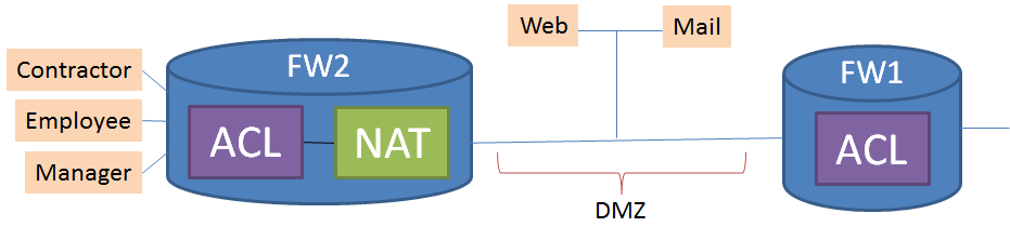
Within the system, NAT maps all addresses to a single static IP address, while the packet filter on firewall2 contains the following rules: :
Deny traffic from DMZ
Deny contractorPC to mailserver
Accept other traffic to mailserver
Accept to webserver on port 80
Assume you’re the sysadmin, and you get a complaint that the manager’s PC is unable to connect to the web. Looking at the architecture and the rules, do you see why this problem has occured?
The problem is that the filter in FW1 is checking for the pre-NAT address from FW2, not the translated NAT address. You could have used Margrave to narrow in on this problem if you couldn’t figure it out from the diagram and rules (indeed, on a larger example, this is just the sort of situation that a tool is useful for!). We actually want to use this example to show you a different Margrave feature, however, one that again asks you to reflect on what formal tools can and should do to help their users. If you want to play with this example yourself in Margrave, here are the files [fw1 filter | fw2 filter | fw2 nat | vocabulary].
How might the sysadmin fix the configuration to give the manager’s PC access to the web? There are many options. One easy option is to change the packet filter on FW1 to use the static IP address that the manager’s PC translates to under NAT. Rules for this solution are in a separate policy file. Is this a good solution? More generally, how might analysis tools help a sysadmin decide whether this is a good solution?
Exercise: Write down a check or computation that an analysis tool might provide to determine whether this is a good solution
One obvious suggestion is to use the tool to verify desired properties of the new configuration, but that has two shortcomings:
It assumes that you have desired properties
It focuses on the entire new config, not the fix (the original question asked about the fix)
In our case, we know that the manager wants to access the web. We could verify that property of the new configuration easily enough using Margrave. But if our goal is to assess the change we made, we probably want to know more than "the reported problem no longer happens". In particular, we want to know what affect the change had: perhaps we broke something while making the fix!
The formal analysis that we really want in this situation is something we call change-impact analysis: we want to give Margrave two policies and ask it to report differences in what the policies allow. If there is a request that one policy accepts and one rejects, we want to know about it. Requests that are treated similarly by both policies aren’t as interesting for assessing the effect of changes. Focusing on the changes limits our attention to the fix, rather than to the new configuration by itself.
Let’s use Margrave to run change-impact analysis on our original and new policies. We load both policies, then write the following query to produce scenarios illustrating changed outcomes:
// the original configurations |
LOAD POLICY aclfw1 = "inboundacl_fw1.p"; |
|
// the revised configuration for firewall1 |
LOAD POLICY aclfw1fix = "inboundacl_fw1_new.p"; |
|
// The COMPARE command defines a query to compute differences |
// between the two named policies over the same inputs |
COMPARE diff = aclfw1 aclfw1fix (interf, sa, da, sp, dp, pro); |
|
show diff; |
COMPARE is just shorthand for a query that we could write manually. The following formula computes the differences between two configurations with permit and deny decisions:
config1:permit(<vars>) and (not config2:permit(<vars>)) or |
config1:deny(<vars>) and (not config2:deny(<vars>)) |
COMPARE simply builds this formula automatically, taking the set of decisions from the vocabulary (it requires that the configurations being compared use the same vocabulary).
This query compared the old and new filters, but did not account for NAT. Since the manager’s failure to reach the web resulted from a combination of filtering and NAT, we should compare the old and new sets of rules in the context of NAT.
This raises a question: how do we hook up the firewall filter and NAT within Margrave? Real systems are connected either with physical wires or with protocols that transmit the same data from one device to another. We can use shared variables to capture each situation. For example, the following formula computes translated addresses for packets permitted by a packet filter:
aclfw2:permit($fw2int, sa, da, sp, dp, pro) and |
natfw2:translate($fw2int, sa, da, sp, dp, pro, tempnatsrc) |
translate is the decision in the NAT configuration for packets that the NAT is willing to handle. If you want details on how NAT rules are defined in Margrave, you can look at the .p file for the NAT configuration. The filter’s permit and NAT’s translate decisions are based on the same variables for the packet contents. The NAT configuration has an additional variable (tempnatsrc) which holds the translated address.
Using a parameter for the result of a computation is a common technique in relation-based modeling. It drives home a key difference between programming and analysis based on model finding. In programming, we execute functions to compute answers and all parameters are inputs. Model finding, in contrast, looks for values of the parameters that satisfy the formula, but doesn’t distinguish between "input" and "output". Relation-based model finding is all about constraints on variables. Using the same variable in two expressions naturally "hooks up" configurations.
Now that we see how to connect the filter and NAT, we can set up the difference query. We are interested in the difference between the old and new queries at the interface between the DMZ and firewall FW1, for packets whose source address results from NAT. The following query uses the previously-defined diff query to look for differences between the old and new versions of FW1, for IP addresses other than the manager’s PC. In the query, $fw1dmz is a constant naming the interface between FW1 and the DMZ (it is defined in the .v file):
let fullci[sa: IPAddress, da: IPAddress, |
sp: Port, dp: Port, pro: Protocol, |
tempnatsrc: IPAddress] be |
|
// topology: packet passes filter and sa NATs to tempnatsrc. |
aclfw2:permit($fw2int, sa, da, sp, dp, pro) and |
natfw2:translate($fw2int, sa, da, sp, dp, pro, tempnatsrc) and |
// look for diffs between original and fixed versions of FW1 |
diff($fw1dmz, tempnatsrc, da, sp, dp, pro) and |
// limit to internal source addresses and external destinations |
InternalIPs(sa) and OutsideIPs(da); |
|
SHOW fullci; |
The scenario produced indicates which packet contents are handled differently, but it is not clear which of the two policies permitted and which denied. We can get that information using the include directive to the show command, asking to see which decisions were rendered (they appear in the bottom-most segment of the scenario):
SHOW fullci |
include aclfw1:permit($fw1dmz, tempnatsrc, da, sp, dp, pro), |
aclfw1:deny($fw1dmz, tempnatsrc, da, sp, dp, pro), |
aclfw1fix:permit($fw1dmz, tempnatsrc, da, sp, dp, pro), |
aclfw1fix:deny($fw1dmz, tempnatsrc, da, sp, dp, pro); |
If we look at the resulting scenarios, we see that source addresses other than the manager’s PC are able to access the web. Whether this is good or bad depends on the organization. If the goal is to have only the manager access the web, this is not a good change. Otherwise, this could be fine. Note that this points out a useful trait of scenario-based analysis: the tool doesn’t provide the judgement of whether this is a good or bad change. That is up to the configuration author to decide upon seeing the scenarios.
Let’s assume that we did not want anyone other than the manager to get access to the web. In that case, we might want a new filter on FW2 that denies web access to non-managers. We could run change-impact analysis to compare this new policy to the original, and indeed over the first several scenarios it would seem that only non-managers have been affected. Still, we would like to confirm that our change did not affect the manager. We don’t want to have to manually inspect all the scenarios to check this. Instead, we’d like to verify a property of just the change scenarios: specifically, that we did not change access for the manager.
We’ve already shown you everything you need to do this: you need to create a diff predicate with the filter for FW2, then create a query that asks for scenarios that satisfy diff and come from the manager’s PC. If Margrave produces no scenarios for this query, then the change does not affect the manager’s PC.
LOAD POLICY aclfw2 = "inboundacl_fw2.p"; |
LOAD POLICY aclfw2fix = "inboundacl_fw2_new.p"; |
COMPARE diff2 = aclfw2 aclfw2fix (interf, sa, da, sp, dp, pro); |
|
let fw2ci[sa: IPAddress, da: IPAddress, |
sp: Port, dp: Port, pro: Protocol] be |
diff($fw2int, sa, da, sp, dp, pro) and |
$managerpc=sa; |
|
poss? fw2ci; |
Margrave returns false, which confirms that the changes do not affect the manager.
Of course, you might also want to verify that the final configuration containing the fixed FW1, original NAT, and fixed FW2 does indeed let the manager access the web but not the others. We could do this in two queries (one for the manager and one for the rest), as shown in the script file (query names managerblocked and nonmanager).
Note that change-impact helped us identify the second of those queries. Originally, we set out to give the manager access: we had not stated a requirement about the non-managers. The change-impact scenarios reminded us that non-managers could be affected, which in turn suggested a property to verify of the final configuration. This is a terrfic use case for change-impact: explore without properties to understand the space, then write properties to check for desirable or undesirable situations that arise in the scenarios.
The point of this segment was not just to show off change-impact as a nice Margrave feature. This segment asks you to think fundamentally about the relationship between "formal analysis" and "verification". "Verification" assumes that you are comparing a configuration and a property. That’s fine when you have a property, but people often don’t have properties! Perhaps they never wrote them down, or they don’t know what to ask, or they don’t have time to think that through carefully.
Change-impact analysis illustrates that you can apply formal methods whenever you have two concrete artifacts to compare: in this example, we had two concrete configurations (rather than a configuration and a property). If you are building a formal analysis tool, ask yourself what artifacts you can expect your audience to have. Ask yourself what workflow they are in when they could use a formal tool. Then try to design an analysis that works with existing data. Change-impact does that for situations in which we have multiple configurations.
This segment has introduced change-impact analysis, which computes the semantic difference between two policies. There are several key takeaways from this segment:
Properties are not required for formal analysis. One can define a formal analysis to compare any two artifacts. Change-impact works on two configurations.
Many use cases provide multiple configurations. This example looked at fixing a configuration to change behavior. Other use cases include refactoring (analysis can confirm that behavior has been preserved) and understanding the tradeoffs between two approaches to writing an original configuration.
Writing a configuration as multiple policies (in this case, one for NAT and one for filtering) provides flexibility during analysis: you can analyze edits to specific parts, then check their impact on the configuration overall.
Variables are a good way to connect multiple policies into a larger configuration.
4 Modeling Complex Boxes through Decomposition
So far, we’ve taken small, specific examples and showed you how to work with them in Margrave. What if your ultimate goal is to use Margrave (or a similar tool) to help process an existing configuration language? For that, you need to understand how to map a complex existing language onto the existing tool. In this segment, we will walk you through an example of how to do that, using Margrave as the back-end tool and Cisco’s IOS language for configuring routers and switches. Our goal is to raise general ideas and strategies you might consider in doing such a mapping.
4.1 Capturing a Complex Configuration
Let’s start with a sample IOS configuration (we’ve added the line numbers for reference) . The following diagram shows the architecture: the system has a firewall with two named interfaces, with the external interface connected to a server:
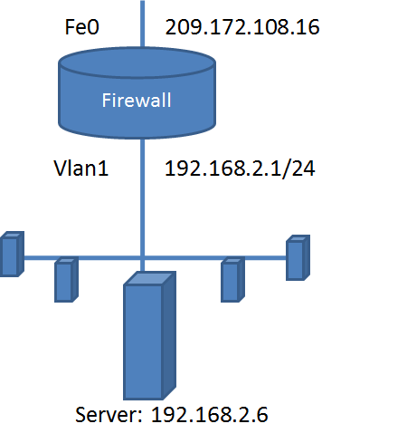
The IOS configuration covers several different tasks internal to the firewall. Let’s briefly show the correspondence between parts of the configuration and the tasks . As we can see, this configuration does a combination of filtering, NAT, routing, and switching. Now, our task is to capture this configuration in Margrave.
Exercise: You’ve seen Margrave’s core language: rules that state decisions for conditions. Take a few moments and discuss what decisions you need to capture this configuration in Margrave, roughly what data goes into the rules for those decisions, and roughly how you will group rules into Margrave policies.
Hopefully, you are realizing that the multiple tasks within an IOS configuration don’t naturally belong within the same set of rules. Earlier, we created separate policies for filtering and NAT; perhaps we should do the same for switching and routing. Actually, if you dig carefully into IOS policies, you’d find that there are nine separate stages with independent rules, co-mingled in a single configuration! The following diagram shows the stages :
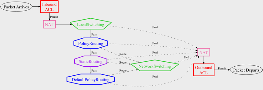
We capture IOS configurations in Margrave by creating one Margrave policy for each of these stages (note that there are separate filter/access-control (ACL) and NAT policies for each of inbound and outbound traffic). The decisions supported by each policy are shown on the diagram .
Exercise: What are the advantages and disadvantages to creating a separate policy for each of these components, rather than one single policy encompassing everything?
Separation of Concerns (advantage): it naturally clusters rules for related decisions together
Fine-grained Granularity (advantage): separate policies for each stage make it easier to reason about individual stages (how would you reason about just the filtering rules, for example, if they were embedded within a larger set.
Simpler language and/or rule combinators (advantage): If all of the rules are encoded together, we would need to express rule combinators on subsets of rules, which would complicate the rule-combination language. Similarly, we would probably need ways to encode the topology by which data from one set of rules flows into another. Since this can’t be expressed directly in rules, we would need to complicate the policy language to capture this.
Need to produce and manage multiple files (disadvantage): this is annoying, but in reality we write compilers to translate from a source language to the back-end, which helps with the production side (Margrave havs an IOS compiler, for example).
Overall, by being willing to decompose the single IOS configuration into multiple Margrave policies, the individual Margrave policies are simpler, cleaner, and more flexible. This is an important takeaway from this session: decomposition is often essential to making a good formal analysis tool. If the language you want to analyze is more complicated than the back-end tools support, look for a good decomposition.
Of course, decomposing IOS into multiple Margrave policies still leaves a gap: somehow, we need to connect the policies into an overall configuration.
Exercise: Stop and think: Where could we connect the nine policies into one firewall? Does this go into a Margrave .p file? Somewhere else?
Remember that we did this in the previous example with filtering and NAT. We used shared variables to create links from one policy to another, using logical and to create a larger logic expression including each component. Do you remember where that and expression was written down? The .p file? The .v file? Neither: the expression to link policies into a whole configuration was embedded in the queries that we sent to Margrave. We introduced variables for the packet contents, then used those variables both to link policies into components and to state the conditions for our query.
Let’s sketch out the topology expression for a subset of the IOS stages. In particular, let’s take the portion consisting of DefaultPolicyRouting, NetworkSwitching, outbound NAT, and outbound packet filtering (ACL):

We’ll use our earlier topology encoding example as a guide. In that example, we had a packet filter flowing into a NAT, with the resulting expression
aclfw2:permit($fw2int, sa, da, sp, dp, pro) and |
natfw2:translate($fw2int, sa, da, sp, dp, pro, tempnatsrc) |
Note that in this topology, there was only one flow from one policy to another: that from the filter to NAT on a permit decision. In our IOS subset, DefaultPolicyRouting goes to different policies depending on the decision: a route decision sends the packet to NetworkSwitching, while a Fwd decision sends the packet to the outbound NAT. So the real question here is figuring out how to encode different connections from the same policy in formulas.
Exercise: Sketch out the formula you would use to capture our IOS policy subset. Don’t worry about the detailed parameter names just yet. Use the policy names as predicates and just figure out the high-level shape of the formula capturing the topology.
Here’s a sketch of the formula. iIn and iOut are the entry and exit interfaces for the packet, host is the hostname, and the other variables have been as in previous queries.
// Option 1: the default policy route specifies an interface: |
(DefaultPolRoute:forward(host, iIn, sa, da, sp, dp, prot, iOut) |
OR |
// Option 2: the default policy route specifies a next hop: |
DefaultPolRoute:route(host, iIn, sa, da, sp, dp, prot, next-hop) |
AND Networkswitching:forward(host, next-hop, iOut) |
OR |
// Final option: Packet is dropped because no policy applies. |
DefaultPolRoute:pass(host, iIn, sa, da, sp, dp, prot) |
AND Interf-drop(iOut) ) |
|
// Finally, the outgoing ACL and NAT apply: |
AND OutboundNAT:translate(host, iIn, sa, da, sp, dp, prot, |
sa2, da2, sp2, dp2) |
AND OutboundACL:permit(host, iOut, sa2, da2, dp2, dp2, prot); |
Roughly speaking, each path through the topology is represented by an and-expression, with those expressions combined with or. We have refactored the expression to share common terms across the paths (reflecting the structure of the graph). We don’t expect you to get the details, but you should get the general idea of what the graph looks like encoded as a formula: a particular path gets taken if the expressions that make up the path can all be satisfied with bindings for the variables.
This gives you an idea of how to set up topology encodings. Since every IOS configuration follows the fixed topology shown in the earlier figure, Margrave’s IOS parser automatically defines the topology query. This means that someone using Margrave to analyze IOS does not need to write the topology query manually; instead, they can just use it in a query (details are in the Margrave documentation). Exporting queries such as this is straightforward, so other projects that compile custom language to Margrave can easily do the same.
Let’s step back for a moment. Putting the topology of policies into queries, rather than into the configuration, seems odd on some level: why is a query a good place to do this? And doesn’t that mean a lot of repeated code across queries (especially for large topologies)?
Putting topology into queries offers two main advantages:
flexibility, in that you can decide which versions of components to hook up on a per-query basis (useful for change-impact analysis, for example). Being able to refer to specific subtasks within a larger configuration is extremely useful during analysis and debugging.
the policy language stays simple, which usually makes analysis more efficient (performance-wise).
The reuse question raises an important concern. Analysis tools can and should provide support for reusing definitions and queries (not just for this situation). Earlier, we showed you the let construct in Margrave, which defined formulas. We can use let to define a reusable topology over multiple policies.
4.2 Queries over Complex Topologies
Queries over complex topologies look no different from queries we have already seen. You can use a let statement to name the topology, then use it in a query. For example, Margrave automatically defines a query called passes-firewall to capture a packet passing through the entire topology. It also exposes a name for each component of the topology. Queries can therefore look at either local portions or the entire scope of the configuration, using expressions such as:
passes-firewall(hostname, entry, sa, da, sp, dp, protocol, paf, |
exit, sa2, da2, sp2, dp2) and |
LocalSwitching1:forward(hostname, da2, exit); |
Our goal in this segment has been to give you a taste of how to think about using an existing tool like Margrave with an existing configuration language. Our emphasis has been on how to decompose configurations into pieces of an appropriate granularity, and on one flexible approach to hooking components into a larger configuration.
5 Wrap Up
Our session has had two broad goals: to introduce you to Margrave (our particular policy-analysis tool), and to give you ideas to think about should you want to build an analyzer for your own language. Both Margrave and all of the configurations and scripts we worked with today are available for you to experiment with at http://www.margrave-tool.org/cornell-13/margrave-install.
As you go forward with formal methods, here are the big-picture points to keep in mind:
If you want to analyze both behavior and structure, you have to model your configurations in a way that exposes the structure through named concepts, as we did for Margrave’s policy rules.
Formal analysis does not require user-defined properties, which can be hard for users to formulate. If you have at least two well-defined artifacts, you can probably write an analysis to compare them. Change-impact is one form of property-free analysis.
Decomposition is essential to making analysis flexible and computationally tractable. Before you encode your language in a tool, ask whether your language can be decomposed into pieces, some of which get handled in queries. For IOS, we used two kinds of decomposition: one separated rules from topology, the other partitioned rules into meaningful subunits. We used Margrave’s policy language to capture each subset of rules, and embedded topology within queries.
Building an intermediate language for your domain can give you a lot of flexibility in defining analyses later. One of our early Margrave prototypes was written directly in Alloy, but that direct encoding was complicated and inflexible once we wanted to start reasoning about rule structures. By creating Margrave as an intermediate language, we made it easier to think about what Margrave needed to do, tweaking the compiler from Margrave to its back-end (which is Kodkod, the back-end underlying Alloy rather than Alloy itself).